Developable Plate Ruling Line Example
Stephen M. Hollister
New Wave Systems, Inc.
www.newavesys.com
This example or tutorial
covers the following topics: reverse engineering (getting existing geometry
data into the program), fairing or smoothing curves, creating developable
surfaces using our unique dynamic ruling line capability, and plate layout or
development. If you are new to computers or new to computer-aided design, you
should really start with another of our tutorials, called “CreateBoat”. The CreateBoat
tutorial covers the easiest way to start a boat design process using the
principal dimensions of the boat. This tutorial covers most all of the other
ways of defining your shape.
This tutorial describes
how I recreated a traditional rowing dory whose offsets (defining data points)
were taken from Skene’s Elements of Yacht Design, by Francis S. Kinney (Eighth
Edition, 1973, pg 47). This rowing dory is 12 feet long and consists of three
surfaces or panels and four edge curves: the sheer or deck edge, the upper
chine, the lower chine, and the keel line. Each edge curve is defined by a
series of [X,Y,Z] points (offsets). X is a measurement along the length of the
boat (starting at the bow or the forward end of the waterline and increasing
towards the stern), Y is the half breadth or width measurement, and Z is the
height measurement. It was designed (before computers) to use plywood for
construction.

Final rendered 3D view of the dory
Reverse Engineering or Geometry Input
These are the things you
can do if you have an existing shape (or idea of a shape) that you wish to get
into the program.
First, you can read in the geometry data from another
program using a standard transfer file format. Our programs accept DXF, IGES,
and TXT file input. The TXT or text file input can be used to transfer geometry
from a spreadsheet to our program. Also, if you have one of our boat design
programs (ProSurf , ProBasic, or ProChine), you can read various standard hull
offsets files, like GHS, NWS, OFF, and SHCP. These files use offsets to define
a series of stations or sections along the length of the hull.
The DXF file is one that
is defined by Autodesk for their AutoCAD program. It has become a standard way
to transfer simple geometry like points, lines, polylines (a polyline is a
series of points connected by straight lines), and curves. The IGES (Initial
Graphics Exchange Specification) file format is more complete than the DXF
format and can be used to transfer more complex geometry like NURB surfaces.
If you have your
geometry in another program and you want to get it into one of our programs,
look to see if your program can output your geometry into an IGES or DXF format
file. If so, then try one of those formats to see if you can read it into our
program. You can check our manual in the “Help” section of the program under
“File” to find out all about each of these formats. Call us if you need further
help.
If your geometry data is
in a spreadsheet or if you have your own special application that creates the
geometry, then you want to look at our own TXT file format that is easy enough
for anyone to understand and use. [See also our article called: Reverse
Engineering 3D Computer Hull Shapes From 2D Lines Drawings and Offsets Tables,
which includes an example of transferring geometry from a spreadsheet to our
program.]
For example, the
following picture shows the partial contents of a TXT file (in our format) that
defines two polylines (connected points) in three dimensions (using X,Y,Z]. The
first line of the file has the label “PLINE3D”. The second line states the
number of points as: “Npts= “. The following lines contain each of the X,Y,Z
points of the polyline, one point per line using blanks to separate the
numbers. Blank lines are ignored and you can put as few or as many geometry
definitions in the file as you want. The “Help” command in the program under
File explains all of the input and output file formats in detail.
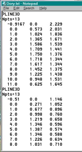
Example of our TXT file for geometry input
Second, you can input the data directly by typing in
the numbers. Whenever the program is asking for you to pick the left mouse
button to define a point (a point entity, a curve or polyline point, or a point
on a surface), you can instead type in the [X,Y,Z] coordinate with the keyboard using the following format:
X,Y,Z
For example:
2.5,3.732,1.5
… to define a point at
X=2.5, Y=3.732, and Z=1.5
As you type in these
numbers they will appear on the status line at the bottom of the screen and the
program will use that point when you press the enter key. This method is useful
if you have a limited set of coordinates or offsets that you want to get into
the program. You could do many input points this way, but you might find it
easier to use a text editor, like NotePad or a spreadsheet, like Excel.
A variation of this
technique is to first define the curve using the number of points for which you
have offsets or coordinates. Then you can pick each point using the right
mouse button and a dialog box will appear (see below) showing the current X,Y,Z
values for the point and allowing you to change or set the new, desired value.
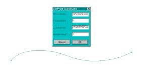
This dialog box appears when you right click on
an edit point.
If you have a lot of
points to enter, then typing them into a text file with NotePad using our TXT
format is probably the fastest method.
Third, you can input the geometry using a 2D digitizer
tablet if you have a paper drawing that defines the geometry. 2D digitizers
come in all sizes, but the most common one is approximately 12” X 12”. You tape
your drawing to the digitizer and enter the curve shape into our program using
your drawing as a template.
Fourth, you can use a 3D digitizer arm (MicroScribe,
Faro Arm, etc.) to directly get the shape into our program. Most of these 3D
digitizers can generate a text form of the digitized point that can be passed
to our program. Our program will treat the point values exactly the same as if
you typed in the values.
Fifth, you can use 3D scanners (laser or otherwise) to
generate a cloud set of points that define the shape of the object. The problem
is that these techniques usually generate hundreds, thousands, or even millions
of points on the object. Our program can read these points, but you still have
to fit the curves and surfaces to these points manually. This can be done by
snapping cross-section curves to some areas of the cloud of points and then
fitting a surface to these curves. This is more tedious than automatic surface
fitting techniques, but you end up with surfaces that you can use to do fairing,
smoothing, or other shape alterations.
Starting the Program
Double click the program
icon on your desktop. The default display shows four screens for four different
views of the model. Although this was recommended to me as being the common CAD
approach, I like to work with one large view at a time. That is why I always
delete 3 of the 4 windows and maximize the last one. (Actually, you can set
this one window display as the default display by changing the “Set4Views”
parameter in the program’s “INI” file to “n”. Many programs have “INI” files
for setting default program values. Look for the ProSurf.ini, the ProBasic.ini,
or the ProChine.ini file in your Windows folder.
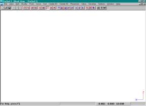
This is what the program looks like with only one (empty) view on the screen.
The data that I need to
get into the program is from an offsets (coordinates) table in the eighth
edition of Skene’s Elements of Yacht Design (1973), on page 47. Unfortunately,
the coordinate values are defined using feet-inches-eighths and I had to
convert them all to decimal feet. I have a simple program to do that, but I
still had to type them all in by hand. The end result is the TXT file shown
above containing the 4 chine curves for the boat. These curves define the edges
of each of the panels that will be used to create the boat. This boat was
designed to use developed plates, so we will see what the program says about
the developability of these panels.
Reading in the Geometry Data
I used the File-Data
File Input-TXT File Input to read the TXT file. The result of this file read is
shown below.
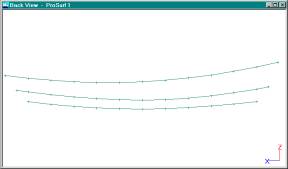
Profile or Side View of Curves
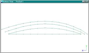
Plan or Bottom View of Curves
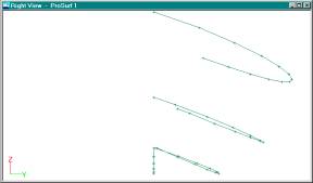
Section, Right, or Bodyplan View of Curves
Remember that the TXT
file contained polylines, which are a series of coordinate points that are
connected by straight lines.
NOTE - Our program uses the term “curves” to refer to
any combination of curve and polyline. Most CAD or drawing programs define
separate entities or geometry types for polylines and curves. This makes it
difficult to deal with shapes that are a combination of smooth, curved portions
and hard, knuckle points. It also means that you have to create, edit, and
delete these entities separately. Our program assigns a special indicator for
each edit or defining point that tells the program whether the line passes
through the point like a smooth curve (or batten) or as a hard knuckle point.
If all of the points are defined as hard knuckle points, then the “curve” is a
polyline. If all of the points are defined as smooth curve points, then the
“curve” is a smooth curve.
It is very simple for
the user to change the smoothness indicator value of any curve defining point
with just one command. This is done with the Curve-Knuckle Pnt command. If you
use this command to “click” on an edit point, it will toggle the status of that
point back and forth between being a smooth curve point and a hard polyline
point. When you use the Curve-Add Curve command, the points will be entered as
smooth curve points. You can override this by using the ‘k’ (knuckle) key to
“pick” a point rather than using the mouse button. If you use the Curve-Add
Polyline command, the points will be entered as hard knuckle points. You can
override this by using the ‘c’ (curve) key to “pick” a point rather than using
the mouse button. After you create the curve, you can still change the
smoothness status of any point using the Curve-Knuckle Pnt command. You are not
stuck with the values you used when you created the curve. Often, users will
define a rough shape of an object using a simple polyline. Afterwards, the user
will selectively convert some of the hard, knuckle points to smooth curve
points while doing the final shaping and fairing. There is no need to deal with
more than one geometric entity as in most other CAD programs.
Editing and Fairing the Curves’ Shapes
As shown below, try
moving one of the points (see the Move Pnt command on the toolbar) to see that
everything is connected by straight lines; not curves. This is something you
always have to watch out for, since many programs transfer the shape of curves
(via DXF, IGES, etc.) as polylines defined with very many points. It looks
smooth like a curve, but it isn’t. You
can check for this by moving a point and seeing if it looks like the picture
below.
Move a Point to See if the Curve is Really a Polyline.
Use the Undo command to
undo this change in curve shape.
Before we can check the
smoothness of these curves, we first have to convert them to real curves with
smoothness. This is done using the Curve-CurveFit command. After applying this
command to each of the curves (use the bottom or right view), try moving a
point to see what happens, as shown below.
Move a Point to See That the Curve is Now a Smooth Curve.
Now you can see that
each of the curves is a true, smooth curve and not just a connected set of
lines. The next step is to use the program’s curvature overlay curve to check
on the fairness or smoothness of these curves.
Use the Undo command to eliminate this shape change.
The big problem with the
computer screen and smooth curves and surfaces is that you cannot tell (by
looking) whether a curve or surface is smooth enough for your application. That
is why our program uses a unique overlay curvature (in orange) that magnifies
all minor little bumps, wiggles, and inflection points.

Profile View Showing Orange Curvature Curve Overlay.
The orange curvature (or
K-curve) in this view was drawn using the Curve-K_Curve Toggle command (which
is the same as picking the ‘K’ icon on the toolbar). This command acts like a
toggle or on/off switch. One click on the curve and the K-curve turns on and
another click on the curve and the K-curve turns off. When you move a point on
the curve, the shape of the curve and K-curve both change shape. The K-curve is
designed to change shape dramatically when the curve is moved just a little
bit. This allows you to “see” very small changes in curve shape even on a small
computer screen. What this also means is that if the K-curve looks smooth, then
the curve it relates to must be very smooth. Remember that smoothness or
fairness is human judgment and you will have to decide when the curve or
surface is smooth enough. This will discussed in more detail later.
If you use the regular
Edit-Move Point command for one of the edit points, you will see that the
K-curve changes dramatically with just a small change in curve shape. That is
why the program has a fine-tune command called the Edit-Move Point % command
(see also the % sign with the 4 arrows on the toolbar). This command works
exactly like the regular Move Point command, except that the point is moved
only 1/100th (1 percent) of the distance in the direction of the
cursor. When you use this command, you may not see the curve move much, but you
will see the K-curve move. That is the whole idea of how this fine-tune fairing
or smoothing works.
Try using the regular
and fine-tune Move Point commands on a curve with the K-curve turned on and
watch how the orange K-curve changes shape. You should see that the Move Point
% command gives you the required fine-tune shape control over the curve. This
allows you to fair the curve without having to zoom in on the curve.
K-Curve showing Unfairness and Inflection Points.
This picture (profile view
of the dory curves) shows you how much the orange K-curve changes shape with
just a small change in curve shape. Another thing to notice is that whenever
the K-curve crosses the curve, it defines an inflection point in the curve – a
place where the curve changes from convex to concave in shape. Remember, for
fairing or smoothing, the goal is to make the K-curve smooth without a lot of
up and down jagginess of the K-curve. However, you will find that there are
many ways to make the K-curve smooth. You have to decide how to fair the curve.
As one of my professors used to say in the days of hand drafting with splines
and battens: “Don’t let the batten design your boat”. Therefore, I will say:
“Don’t let the K-curve design your boat”.
K-Curve Shown in the Plan or Top View.
This picture shows you
the curves and K-curve in the plan (or top or bottom) view of the boat. You
have to fair or smooth the curves in all views. For these curves, that run the
length of the boat, you really just want to fair them in the profile and the
plan views. If you display the section or bodyplan view of the boat, then the
K-curve will be exaggerated too much due to the foreshortening of the curves.
Generally speaking, you want to fair the longitudinal curves in the plan and profile
views and you want to fair the sections (transverse curves) in the section or
bodyplan view.
K-Curve Shown With Reduced Magnification.
How do you know if the
curve is fair enough? It is a judgment call, but there are a few rules to
follow. First, the K-curve is relative. You can increase or decrease its
magnification using the K-up arrow or the K-down arrow buttons on the toolbar.
The shape of the K-curve will not change – just it’s magnification. These two
buttons turn up or down the magnification of the K-curves by a certain amount.
You can keep clicking on the button to keep increasing or decreasing their
magnitudes. The picture above shows what happens to the K-curve in the plan
view when you use the K-down arrow button a few times. When you turn the
K-curve down too much, it does not change shape much and it is less sensitive
to the changes using the Move Point % command. When you turn the K-curve up too
much, it changes too much even with a tiny change to the shape of the curve.
What you want to do is to magnify or reduce the K-curve until it changes a
little bit if you change the shape of the curve by the building tolerance.
For example, if you are
building a boat and the best accuracy you need is about 1/32nd of an
inch, then you want to adjust the sensitivity of the K-curve until you can see
changes in the K-curve when you move the curve by 1/32nd of an inch.
If you lower the magnification any more than this, you will no longer be able
to smooth the curve to within the building tolerances. You can look at the
status line when you are using the Move Point % command to see how much you are
moving an edit point. When you move an edit point by the building tolerance,
you should be able to see a slight change in the K-curve. On the other hand, if
you magnify the K-curve too much, you will see wild changes in shape of the
curve even when you move an edit point by the building tolerance.
Most of the time, the
default magnification works fine and that is what you should use. Try
increasing and decreasing the K-curve magnification using the K-Up and K-Down
toolbar buttons and test it out with the Move Point % command.
K-Curve Shape When the Curve is Finally Faired.
This is the same curve
after it has been faired. Notice that the K-curve is fairly smooth. It doesn’t
have to be perfectly smooth. Remember that the K-curve is a large magnification
of the smoothness of the curve. If you do try to make the K-curve perfect, then
you might end up spending a lot of time smoothing the curve to within a 1/100th
or 1/1000th of an inch.
Profile View Showing all K-Curves at Once.
This picture shows the
K-curves for all four chine curves on the dory. You might want to do this to
compare the shapes of the consecutive curves. The calculations of the K-curves
are independent of each other, but they should all have somewhat the same
shape.
Plan View Showing All K-Curve Lines
This picture shows the
same K-curves in the top (bottom) or plan view. All of the curves (using the
offsets from the book) have been faired to within the building tolerances
Checking Plate Developability
Let’s check to see how
developable the plates or panels are using the program’s ruling line
calculations. Remember that a surface is perfectly developable if it can be
created with absolutely no twisting or stretching of the plate material. In
real life, however, a small amount of twist or double curvature is perfectly
acceptable.
First, let’s get some
background information on ruling lines. What is a ruling line? I will use an
example that perhaps you can visualize. Imagine that you are building the dory
in this example upside down and you have several frames set up along the length
of the boat. Also, imagine that these frames are notched at the chines and
sheer and that you have longitudinal chine and sheer bars or battens that
define these curves. Your job is to lay a piece of plywood across from one
chine curve to another and wrap the plywood to fit the chines and frames.
When you take the flat
sheet of plywood and first lay it down between two neighboring chine curves,
you will notice that the plywood touches the chine curves at only one spot
(assuming that the curves are not flat). If you connect those two chine
touching spots with a line, that line would be a ruling line. If you continue
this process over the entire length of the hull, then you will have a large
number of ruling lines that span the two chine curves. If any of these ruling
lines cross or if you can’t find any ruling lines for a particular section of
the surface, then the surface is considered to be non-developable. Either you
cannot build the surface out of flat material or you might have to stretch
(torture?) the material quite a bit.
Our program tries to
account for different amounts of twist in different materials by allowing for a
certain amount of twist (in degrees) along each ruling line. Let’s go back to
the ruling line example. This time, imagine that you and your helper are on
opposite sides of the sheet of plywood that you laid down across the chine
curves. Both of you go to the spots on the plywood that touch each chine. These
are the ends of the ruling line. At each end of the imaginary ruling line on
the plywood, you both glue a pencil perpendicular to the plywood on top of the
plywood. Now there is a pencil pointing straight out from the plywood at each
end of the imaginary ruling line. Next, you both bend down and look along the
ruling line from one pencil to the other. Since you haven’t bent the plywood
yet, the two pencils should line up exactly – there is zero twist in the ruling
line or in the plywood.
Next, each of you should
grab the plywood on each side of the ruling line and twist the plywood in
opposite directions so that the pencils start to point in opposite directions. You
are introducing twist into the plywood. If you now sight down the ruling line
at the pencils (assuming that you can twist and look down the ruling line at
the same time), you should see that the pencils do not line up. We define twist
as the angle (in degrees) between the two pencils when you sight down the
ruling line. You can tell the program how much of this twist is allowable when
it looks for ruling lines between any two curves. [See the help manual for more
complete details about how the ruling line calculation is done.] The program
will find a set of ruling lines between two curves and draw them using a color
that is related to how much twist is found to be in that ruling line. Dark blue
is used for perfectly developable hull with no twist. As the color changes to
light blue, green, then to yellow and red, the twist gets larger and larger. If
the twist gets larger than some angle limit that you define, the program will
not draw the ruling line. See the article on Plate Development and Expansion for
more details on the difficulties of surfaces with double curvature and twist.
The program
automatically recalculates and draws the ruling lines as you edit (drag) the
shape of the chine curves. The goal is to get a nice spread of ruling lines
that are as close to dark blue in color as possible.
There are two purposes
for ruling lines. The first is to check for developability of the plate and the
second is to define the shape of the surface, since the hull is only defined by
chine curves at this point. To “turn on” the ruling lines between any two
surfaces, use the Develop-Set Ruling Lines for Curves command and you will be
prompted with:
“Pick the first of two
curves”
After picking one of the
two curves (in any order), you will be prompted with:
“Pick the second curve”
Since ruling lines are
calculated and drawn between any two curves, you need to pick both curves to
tell the program which surface or plate you want to work on. You can’t pick
just one curve because each curve can be the edge for more than one surface. If
you use this command for all three dory surfaces, you should see something like
the following.
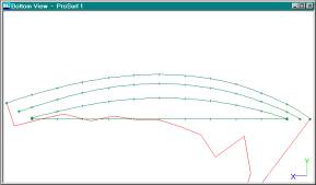
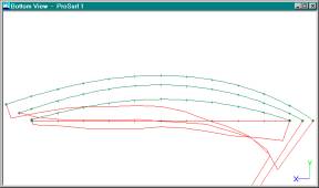
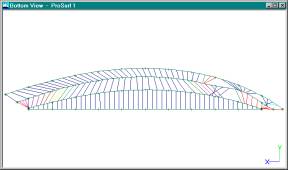
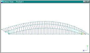
Plan View Showing Ruling Lines Between All Chines
This is the plan or
bottom (bow pointing to the right) view of the dory showing all of the ruling
lines. Remember that the dark blue ruling lines indicate no double curvature or
twist and the areas of green to yellow to red show increasing amounts of twist.
We don’t know yet whether this is going to make the hull unbuildable with plywood.
Since the hull was in Skene’s, I would assume that the developability is close
enough. We will study this later.
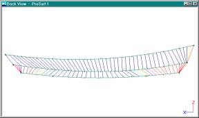
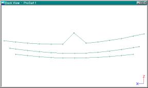
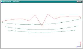
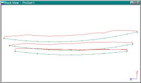
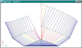
Profile View Showing Ruling Lines Between All Chines
This is the profile or
back (bow pointing to the right) view of the hull showing the same ruling
lines.
If you display the
bodyplan, section, or right view of the hull, you will notice that the
starboard side of the hull is displayed all on one side. What we want to do
(this is not required) is to tell the program where the middle of the boat is
so that the program can “flip” the aft geometry over to the port side for the
section view. This is standard naval architecture practice because it allows
you to see the aft sections without having the forward sections get in the way.
This value can be set using the Options-Display Options dialog box, as shown
below.
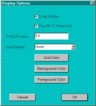
Display Options Dialog Box
Notice that the “X-Flip
Position” is now set to 5, which is in the middle of the boat. When you pick
the OK button, you should see the following for the section view.
Section View With Split View of the Hull
Notice how the forward
sections (ruling lines) are on the right and the aft lines are on the left.
This may take some getting used to, but you will see this layout in all books
about naval architecture. If it really bothers you, then you can change the
“flip” value to some large number, like 2000, to get all of the lines back on
the right.
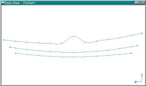
OK, back to the problem
of deciding what is wrong with this hull. You can see some red ruling lines
that indicate twist. But, how much twist is OK? Let’s try a test. Display the
hull in plan (bottom) view and use the Move Pont % command to move a point on
the middle chine in the red region. As you drag the point, see how the ruling
lines change shape. You may see something like what is shown below.
[Note – We probably
shouldn’t have spent much time on fairing the original curves if we expected to
change the shape of the curves to fix developability problems. I would say that
since it is quick to fair the curves, I would initially fair them a little bit,
but I wouldn’t spend a lot of time on it. The assumption is that this is an
existing design that has already been successfully built out of plywood.]
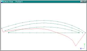
Change in Ruling Lines Due to a Change in the Chine
Notice how things start
to go bad very quickly, even for small changes in shape. This would seem to
indicate that the allowable twist settings are very strict and that maybe this
hull is pretty close to being developable just as it is. [Use the Undo command
to go back to the original shape.] How can we check this out? Let’s look at the
ruling line options for one of the surfaces. The following Ruling Line Options
dialog box can be displayed using the Develop-Ruling Line Options command. When
it is selected, the program asks you to pick the two edge curves of the surface
that you are interested in. When you do that, you should see the dialog box
shown below.
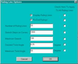
Ruling Line Options Dialog Box
This dialog box allows
you to change a number of options related to one or all of the ruling line
surfaces. The field that we are interested in is the “Desired Twist Angle”
field, which is set to ¼ of a degree. If you remember the description above
about the plywood, the pencils, and the twist angle, then this angle is the
angle between the two pencils. As you can see, ¼ of a degree is pretty strict.
This is the twist angle that the program tries to meet for each ruling line. If
it can’t, then it will find the best ruling line that it can and mark it with
another color, depending on how close it is to the desired twist angle. If the
best twist angle that it can find is greater than the “Maximum Twist Angle”
then the program will not draw the ruling line. This value is set very high
since most people want to see the ruling line anyway and it will be colored
red.
What we can do is to
change the “Desired Twist Angle” to something higher to see what happens to the
ruling lines. Remember, this angle is the twist in the material defined by the
angle between the two pencils. Most people can twist material quite a bit if
they really work at it. However, this twist angle tells the program how much
twist is allowed for all ruling lines. Just because you can locally put a lot
of twist in a surface doesn’t mean that you can do it over the entire surface.
You should be a little bit careful about increasing this angle. If you increase
it too much, then all surfaces will be marked as developable, but the surface
won’t be buildable!
For this dory example, I
think that a 1 or 2 degree twist angle should be fine. Change the “Desired
Twist Angle” field to 2 and pick the OK button.
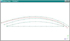
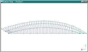
Ruling Lines With a Desired Twist Angle of 2 Degrees
Notice how the ruling
lines look better and that more of the ruling lines are dark blue. If we increase
the twist angle to 3 or 4 degrees, you should see something like what is shown
below.
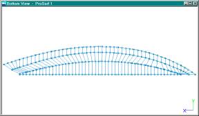
Ruling Lines With a Desired Twist Angle of 4 Degrees
Creating Surfaces From Ruling Lines
It is not necessary to
eliminate all of the ruling lines that are not dark blue. What you do want is a
clean set of ruling lines that don’t wiggle back and forth. This is because we
want to fit a NURB surface across all of the ruling lines. This is done with
the Develop-Fit Surf to Ruling Lines command. When you select this command, you
will have to (like before) select a surface by picking its two edge curves. If
the ruling lines look OK, then go ahead and fit the surfaces to the ruling
lines, as shown below.
Note – There is no exact answer here about how much
twist is allowed in a surface. As you increase the “Desired Twist Angle”, the
program will be able to calculate better and better ruling lines. HOWEVER, this
does not mean that the program says that the surface is buildable.
Just because the program can create the ruling lines and flatten out a surface,
it doesn’t mean that you can take that 2D shape and wrap, twist, and distort
that shape onto the frames without problems. Ultimately, it is your
responsibility to determine if a surface is close enough to true developability
to be buildable. If you have to, print out scale drawings of the 2D patterns
and build a little mock up out of paper or cardboard. Remember, this is only for surfaces with twist or double
curvature. If you have a perfectly developable hull (within a very small twist
angle), then there shouldn’t be any problems at all. Well, I shouldn’t say that
exactly. As described more in the paper on “Plate Development and Expansion”,
even if the hull surfaces are perfectly developable, you still have to be very
careful. One problem is if you wrap the pre-cut plate onto just a few frames.
The plate might not assume the same shape as in the computer program. As you
wrap the plate onto the frames, you might think that everything is wrong. You
have to make sure that you have “enough” frames (even if you have to use
temporary frames) to get the plate to take on the same shape as in the
computer. Another problem happens if you cut out the frames and plates exactly
(by CNC) but someone in the yard sets up a frame slightly canted or in the
wrong location. If everything is cut out exactly, then you have to make sure
that everything is set up exactly. A small error or misalignment in the middle
of the boat can translate to a large error at the ends. There is no more cut
and fit.
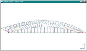
Plan View Showing NURB Surfaces Fit to All Ruling Lines
After you fit the NURB
surfaces to each set of ruling lines, this is what you should see. Now we can
look at the surfaces themselves to see if they are developable. This is done
with the Surf-K_Patch-Kpat All command. This command colors in the surfaces
based on the amount of double curvature (Gaussian curvature) there is in the
surface. The colors are “sort-of” the same as for the ruling lines: dark blue
is for developable surfaces and the colors progress to red for surfaces with a
lot of double curvature. However, the two sets of colors are not calibrated the
same, so the colors only give you a relative idea about the developability of
the surfaces. When you select the command, you should see something like what
is shown below.
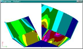
Bodyplan View Showing Gaussian Curvature Colors
The default coloring
fills in just every other pixel on the screen. If you want to see what is shown
above, you need to adjust some options using the Surf-K_Patch-Kpat Options
dialog box, shown below. To get the full saturation of color, you need to
change the Row and Col Density values to 1 and 1. If you pick the OK button,
then you should see the view above.
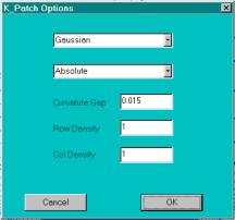
K_Patch Options Dialog Box
Well, the colors look
awful! How can the ruling line method show that the hull is developable
(buildable, anyway) and this display shows lots of non-blue colors. The problem
is that the sensitivity of the Gaussian curvature is not the same as that used
by the ruling lines. If you go back to the above dialog box and change the
“Curvature Gap” value from 0.015 to a larger number and select OK, then you
will see something like the picture below.
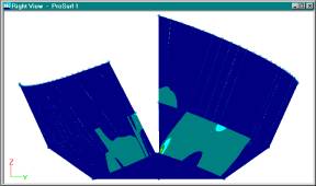
Gaussian Curvature With Lower Curvature Sensitivity
Just by changing the
sensitivity of the calculation, you can show that the surfaces are nearly
developable. Again, if you change the sensitivity up a lot, then anything will
look developable. It is up to you to judge how much twist is allowed before the
surface becomes unbuildable. Generally, I like to use the ruling line twist
angle to judge developability since it seems to have a more real-world or
physical understanding. Gaussian curvature looks nice and is good for a second
check, but I wouldn’t use it as a primary check of developability.
Creating a Developable Hull Shape
This tutorial kind of
glossed over the problem of how you change the shape of the curves if the
ruling lines are not developable. Other programs and an old program of ours
calculated ruling lines only after you made an edit change to one of the curves
and it was extremely sensitive to the slightest change in shape. You were
constantly guessing about what shape change was necessary to get the ruling
lines just right. It was often a painstaking process. Our new technique of
dynamic ruling lines with color-coded twist information is a lot better, but it
isn’t automatic. The sensitivity of the ruling lines can be controlled by the
user, but it is still up to you to know what shapes are developable and what
shapes are not. However, the dynamic ruling lines allow you to check many
different shapes very quickly.
For multi-chine hulls,
you should start at the bottom surface and work up (or at the upper surface and
work down). Get one surface developable and then move on to the next. Changing
the shape of a middle chine (like we did above) is not a great approach, since
it is unlikely that you will manage to get both surfaces developable at the
same time. You have to work on one surface at a time. Over time, you will begin
to get a feel for what shapes are developable and what shapes are not. You will
be able to look at the chine curves and see what has to be done. You can also
start with existing developable designs, like the dory in this example.
Flatten Out the Plates
Finally, once you get
the hull just the way you want and you are ready to flatten out the plates, you
can do so using the Develop-Develop Plate command. It asks you to pick the
surface you wish to develop (just pick one of the surface columns) and displays
the following dialog box.
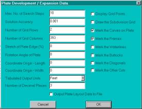
Plate Development Dialog Box
There are a lot of
options here, but try it out using the default settings first. Remember that
the program uses a finite element type of calculation that can work for both developable
and double curvature surfaces. It searches for a reasonable solution, since
there are an infinite number of solutions for surfaces with double curvature.
Many of the options relate to this search process and you can see the full help
manual for all of the details.
When you pick the OK
button, the calculation will be done and you should see a result box, as shown
below.
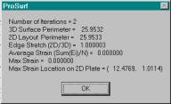
Plate Development Results Box
This result box tells
you that it took 2 iterations to find the solution and that the 2D pattern
perimeter length is almost exactly the same as the 3D perimeter shape of the
surface. (This is a stretch option that can be changed.) It also says that
there is no strain (stretch) in the plate. Everything looks good. When you pick
the OK button, you will see one of the plates shown below.
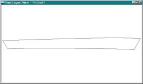
This is the developed 2D pattern for the upper side plate.
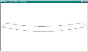
This is the developed 2D pattern for the lower side plate.
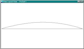
This is the developed 2D pattern for the bottom plate.
Output of the 2D Patterns
You can use the regular
File-Print (see the Print Preview command first) command to print out the
pattern. The default output is to scale the picture to fit the printer paper
you are using. If you want to print it out at a particular scale factor, then
you have to change the settings in the Options-Mod/Doc Definitions dialog box.
If you want to output
the pattern to a DXF file to give to someone else for plotting or CNC cutting,
you have to follow these steps:
- Make sure that the pattern you want to output
is in the current view on the screen.
- Select the File-Data File Output-DXF Output
command. You should see the dialog box shown below.
- Change the top “Output” field to “2D View
Output” to make sure that you output the 2D pattern rather than the full 3D
model of the boat.
- Since you are outputting the 2D view, the
rest of the options really don’t matter. The program will output whatever
is in the current view.
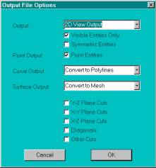
DXF Output File Options
Note that the program
does not scale the numbers (geometry) when they are put into the DXF file. If
you are using feet, the file will contain feet. If you are using millimeters,
the file will contain millimeters. However, the DXF file does NOT contain any
units information so the program that reads the DXF file might assume that the
units are inches. You need to make sure that the receiving program knows what
units you are using.
Frame Shapes and Patterns
I haven’t said anything
about getting the 2D frame shapes of the hull, but now that you have the full
NURB surface shapes, you can define and draw all of the frame shapes. This
tutorial is long enough, so I will just get you going in the right direction.
To get the frame (or station, waterline, buttock, diagonal) shape, you need to
use the PlaneCut commands to define a set of frames, waterlines, buttocks, and
diagonals. The “Initialize Lines” command allows you to define a group of lines
all at once and the Add, Modify, and Delete commands allow you to modify the
initial set of lines. Once the lines are defined, you can turn them on or off
for display and you can display or plot a traditional lines drawing (View-Lines
View) of the hull. Then, you can display and print/plot one or more section or
frame shapes full-size or at any scale factor. You can also send the frame
shapes to a DXF file just like you did for the plate shapes.
3D Views of the Hull
You can also display the
hull in 3 dimensions now that you have the full surface shape of the hull. This
can be done in wireframe or render modes as shown below.
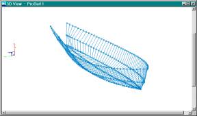
3D Wireframe View of the Hull
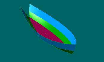
3D Render View of the Hull
Summary
There is much more I
could explain about the program. The goal of this tutorial, however, was to get
you started with the least amount of pain and head scratching. As with any non-trivial
program, it takes some time and patience to master the required skills. I hope
this tutorial makes that task a little bit easier.